search_images_ddg
ims = search_images_ddg('grizzly bear')
len(ims)200This is my follow up to Lesson 2: Practical Deep Learning for Coders 2022 in which Jeremy created a dog | cat classifier model and deployed to Hugging Face. During this project I will try to replicate on an image classification model, which discriminates between three types of bear: grizzly, black, and teddy bears. Once we’ve done this we will proceed to deploy the model as a working app on Hugging Face!
::: {.cell _kg_hide-input=‘true’ _kg_hide-output=‘true’ outputId=‘ba21b811-767c-459a-ccdf-044758720a55’ papermill=‘{“duration”:23.212506,“end_time”:“2022-10-10T06:59:22.512822”,“exception”:false,“start_time”:“2022-10-10T06:58:59.300316”,“status”:“completed”}’ tags=‘[]’ execution_count=1}
! pip install -Uqq fastbook
import fastbook
fastbook.setup_book()
from fastbook import *
from fastai.vision.widgets import *
:::
Now, it’s time to get hold of our bear images. There are many images on the internet of each type of bear that we can use. We just need a way to find them and download them. One method is to use fastai’s search_images_ddg which grabs images from DuckDuckGo. Note that the number of images is restricted by default to a maximum of 200:
search_images_ddg
ims = search_images_ddg('grizzly bear')
len(ims)200NB: there’s no way to be sure exactly what images a search like this will find. The results can change over time. We’ve heard of at least one case of a community member who found some unpleasant pictures of dead bears in their search results. You’ll receive whatever images are found by the web search engine. If you’re running this at work, or with kids, etc, then be cautious before you display the downloaded images.
Let’s take a look at an image:
dest = 'images/grizzly.jpg'
download_url(ims[0], dest)Path('images/grizzly.jpg')im = Image.open(dest)
im.to_thumb(128,128)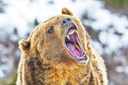
bear_types = 'grizzly','black','teddy'
path = Path('bears')
This seems to have worked nicely. Let’s use fastai’s download_images to download all the URLs for each of our search terms. We’ll put each in a separate folder:
if not path.exists():
    path.mkdir()
    for o in bear_types:
        dest = (path/o)
        dest.mkdir(exist_ok=True)
        results = search_images_ddg(f'{o} bear')
        download_images(dest, urls=results)
Our folder has image files, as we’d expect:
fns = get_image_files(path)
fns
(#295) [Path('bears/grizzly/bd6ab4a5-5126-492d-b69e-bd15e8f8db86.jpg'),Path('bears/grizzly/54c2968d-f1eb-473f-8979-abd2c6a1e9b9.jpg'),Path('bears/grizzly/06c6eeac-94a8-4634-a979-5de67ced9b3e.jpg'),Path('bears/grizzly/6d6c394c-596b-4953-b98c-f90df597d7c1.jpg'),Path('bears/grizzly/d0fb653a-1328-4f3d-95ce-1b5bc588ef04.jpg'),Path('bears/grizzly/b5179606-5957-4a29-8623-fa05ff910ccc.jpg'),Path('bears/grizzly/3e5bb95f-76bf-4847-9c86-a000077fc371.jpg'),Path('bears/grizzly/484483b9-7453-4e08-8487-9066da336bbb.jpg'),Path('bears/grizzly/d39dd49d-669a-4f15-96e7-9476875d859f.jpg'),Path('bears/grizzly/d3f5a27e-a2bc-474a-8acb-afd0708dee20.jpg')...]Often when we download files from the internet, there are a few that are corrupt. Let’s check:
failed = verify_images(fns)
failed
(#5) [Path('bears/grizzly/8ce9dba9-9dc8-4bf3-b392-097b28d86baf.jpg'),Path('bears/grizzly/13127ddd-1639-4b89-b81a-439c43a56fc6.jpg'),Path('bears/grizzly/e537fa0c-c6bf-43f3-acda-024af91b1745.jpg'),Path('bears/black/946c1956-6068-4468-bd3a-10af1fc2ae6a.jpg'),Path('bears/black/001594ba-562a-4ff0-8e3a-d84c654146ea.jpg')]To remove all the failed images, you can use unlink on each of them. Note that, like most fastai functions that return a collection, verify_images returns an object of type L, which includes the map method. This calls the passed function on each element of the collection:
failed.map(Path.unlink);Now that we have downloaded some data, we need to assemble it in a format suitable for model training. In fastai, that means creating an object called DataLoaders.
To turn our downloaded data into a DataLoaders object we need to tell fastai at least four things:
Fastai has an extremely flexible system called the data block API. With this API you can fully customize every stage of the creation of your DataLoaders. Here is what we need to create a DataLoaders for the dataset that we just downloaded:
bears = DataBlock(
    blocks=(ImageBlock, CategoryBlock),
    get_items=get_image_files,
    splitter=RandomSplitter(valid_pct=0.2, seed=42),
    get_y=parent_label,
    item_tfms=Resize(128))
This command has given us a DataBlock object. This is like a template for creating a DataLoaders. We still need to tell fastai the actual source of our data — in this case, the path where the images can be found:
dls = bears.dataloaders(path)A DataLoaders includes validation and training DataLoaders. DataLoader is a class that provides batches of a few items at a time to the GPU. When you loop through a DataLoader fastai will give you 64 (by default) items at a time, all stacked up into a single tensor. We can take a look at a few of those items by calling the show_batch method on a DataLoader:
dls.valid.show_batch(max_n=4, nrows=1)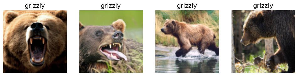
Data augmentation refers to creating random variations of our input data, such that they appear different, but do not actually change the meaning of the data. Examples of common data augmentation techniques for images are rotation, flipping, perspective warping, brightness changes and contrast changes. By default Resize crops the images to fit a square shape of the size requested, using the full width or height. This can result in losing some important details. Alternatively, you can ask fastai to pad the images with zeros (black), or squish/stretch them:
bears = bears.new(item_tfms=Resize(128, ResizeMethod.Squish))
dls = bears.dataloaders(path)
dls.valid.show_batch(max_n=4, nrows=1)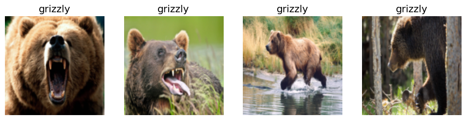
bears = bears.new(item_tfms=Resize(128, ResizeMethod.Pad, pad_mode='zeros'))
dls = bears.dataloaders(path)
dls.valid.show_batch(max_n=4, nrows=1)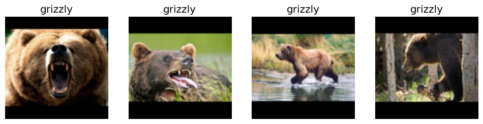
All of these approaches seem somewhat wasteful, or problematic. If we squish or stretch the images they end up as unrealistic shapes, leading to a model that learns that things look different to how they actually are, which we would expect to result in lower accuracy. If we crop the images then we remove some of the features that allow us to perform recognition. For instance, if we were trying to recognize breeds of dog or cat, we might end up cropping out a key part of the body or the face necessary to distinguish between similar breeds. If we pad the images then we have a whole lot of empty space, which is just wasted computation for our model and results in a lower effective resolution for the part of the image we actually use.
Instead, what we normally do in practice is to randomly select part of the image, and crop to just that part. On each epoch (which is one complete pass through all of our images in the dataset) we randomly select a different part of each image. This means that our model can learn to focus on, and recognize, different features in our images. It also reflects how images work in the real world: different photos of the same thing may be framed in slightly different ways.
In fact, an entirely untrained neural network knows nothing whatsoever about how images behave. It doesn’t even recognize that when an object is rotated by one degree, it still is a picture of the same thing! So actually training the neural network with examples of images where the objects are in slightly different places and slightly different sizes helps it to understand the basic concept of what an object is, and how it can be represented in an image.
Here’s another example where we replace Resize with RandomResizedCrop, which is the transform that provides the behavior we just described. The most important parameter to pass in is min_scale, which determines how much of the image to select at minimum each time:
bears = bears.new(item_tfms=RandomResizedCrop(128, min_scale=0.3))
dls = bears.dataloaders(path)
dls.train.show_batch(max_n=4, nrows=1, unique=True)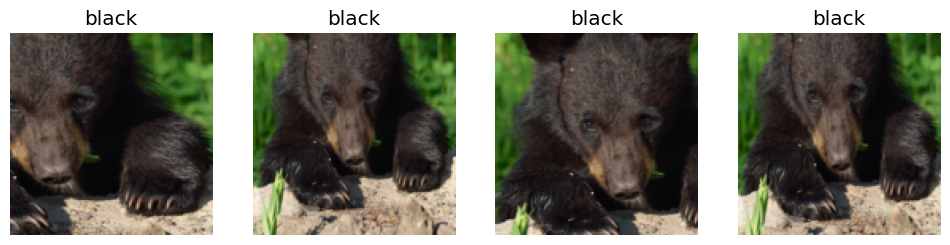
We used unique=True to have the same image repeated with different versions of this RandomResizedCrop transform.
For natural photo images such as the ones we are using here, a standard set of augmentations that we have found work pretty well are provided with the aug_transforms function. Because our images are now all the same size, we can apply these augmentations to an entire batch of them using the GPU, which will save a lot of time. To tell fastai we want to use these transforms on a batch, we use the batch_tfms parameter (note that we’re not using RandomResizedCrop in this example, so you can see the differences more clearly; we’re also using double the amount of augmentation compared to the default, for the same reason):
bears = bears.new(item_tfms=Resize(128), batch_tfms=aug_transforms(mult=2))
dls = bears.dataloaders(path)
dls.train.show_batch(max_n=8, nrows=2, unique=True)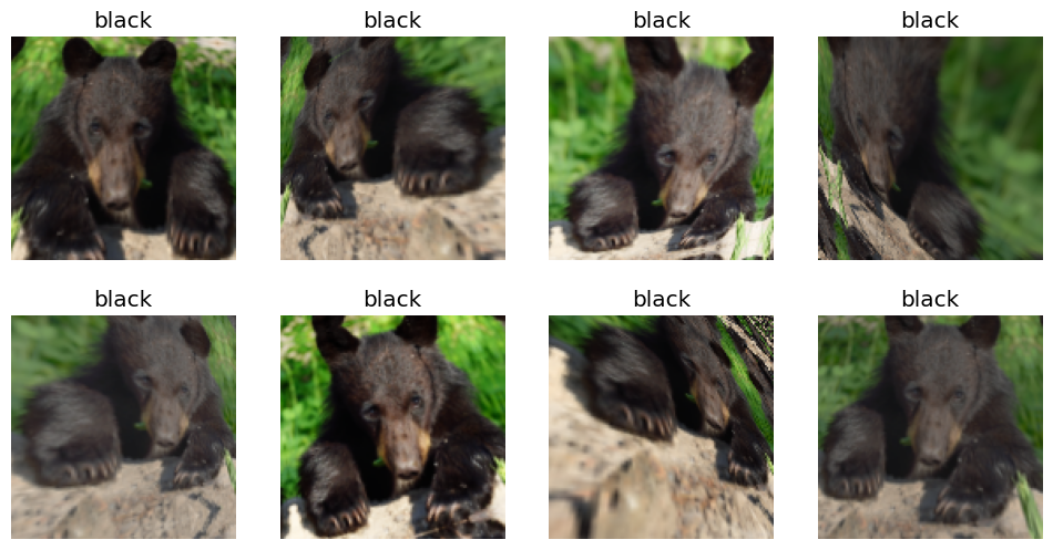
Now that we have assembled our data in a format fit for model training, let’s actually train an image classifier using it.
We don’t have a lot of data for our problem (200 pictures of each sort of bear at most), so to train our model, we’ll use RandomResizedCrop with an image size of 224 px, which is fairly standard for image classification, and default aug_transforms:
bears = bears.new(
    item_tfms=RandomResizedCrop(224, min_scale=0.5),
    batch_tfms=aug_transforms())
dls = bears.dataloaders(path)
We can now create our Learner and fine-tune it in the usual way:
learn = vision_learner(dls, resnet18, metrics=error_rate)
learn.fine_tune(4)
/home/stephen137/mambaforge/lib/python3.10/site-packages/torchvision/models/_utils.py:208: UserWarning: The parameter 'pretrained' is deprecated since 0.13 and will be removed in 0.15, please use 'weights' instead.
warnings.warn(
/home/stephen137/mambaforge/lib/python3.10/site-packages/torchvision/models/_utils.py:223: UserWarning: Arguments other than a weight enum or `None` for 'weights' are deprecated since 0.13 and will be removed in 0.15. The current behavior is equivalent to passing `weights=ResNet18_Weights.IMAGENET1K_V1`. You can also use `weights=ResNet18_Weights.DEFAULT` to get the most up-to-date weights.
warnings.warn(msg)
Downloading: "https://download.pytorch.org/models/resnet18-f37072fd.pth" to /home/stephen137/.cache/torch/hub/checkpoints/resnet18-f37072fd.pth| epoch | train_loss | valid_loss | error_rate | time |
|---|---|---|---|---|
| 0 | 1.192118 | 0.813263 | 0.327586 | 00:11 |
| epoch | train_loss | valid_loss | error_rate | time |
|---|---|---|---|---|
| 0 | 0.407396 | 0.375259 | 0.155172 | 00:13 |
| 1 | 0.308869 | 0.153977 | 0.051724 | 00:14 |
| 2 | 0.247075 | 0.101119 | 0.051724 | 00:13 |
| 3 | 0.217112 | 0.085641 | 0.051724 | 00:13 |
Now let’s see whether the mistakes the model is making are mainly thinking that grizzlies are teddies (that would be bad for safety!), or that grizzlies are black bears, or something else. To visualize this, we can create a confusion matrix:
interp = ClassificationInterpretation.from_learner(learn)
interp.plot_confusion_matrix()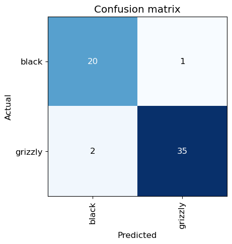
The rows represent all the black, grizzly, and teddy bears in our dataset, respectively. The columns represent the images which the model predicted as black, grizzly, and teddy bears, respectively. Therefore, the diagonal of the matrix shows the images which were classified correctly, and the off-diagonal cells represent those which were classified incorrectly. This is one of the many ways that fastai allows you to view the results of your model. It is (of course!) calculated using the validation set. With the color-coding, the goal is to have white everywhere except the diagonal, where we want dark blue. Our bear classifier isn’t making many mistakes!
It’s helpful to see where exactly our errors are occurring, to see whether they’re due to a dataset problem (e.g., images that aren’t bears at all, or are labeled incorrectly, etc.), or a model problem (perhaps it isn’t handling images taken with unusual lighting, or from a different angle, etc.). To do this, we can sort our images by their loss.
The loss is a number that is higher if the model is incorrect (especially if it’s also confident of its incorrect answer), or if it’s correct, but not confident of its correct answer. In a couple of chapters we’ll learn in depth how loss is calculated and used in the training process. For now, plot_top_losses shows us the images with the highest loss in our dataset. As the title of the output says, each image is labeled with four things: prediction, actual (target label), loss, and probability. The probability here is the confidence level, from zero to one, that the model has assigned to its prediction:
interp.plot_top_losses(5, nrows=1)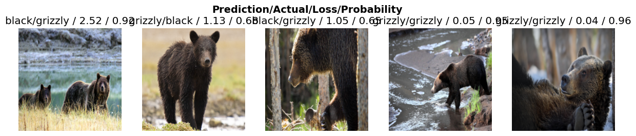
This output shows that the images with the highest losses are ones where the prediction matches the label, however with a low degree of confidence.
The intuitive approach to doing data cleaning is to do it before you train a model. But as you’ve seen in this case, a model can actually help you find data issues more quickly and easily. So, we normally prefer to train a quick and simple model first, and then use it to help us with data cleaning.
fastai includes a handy GUI for data cleaning called ImageClassifierCleaner that allows you to choose a category and the training versus validation set and view the highest-loss images (in order), along with menus to allow images to be selected for removal or relabeling:
#hide_output
cleaner = ImageClassifierCleaner(learn)
cleaner
We can see that amongst our “black bears” is an image that contains two bears: one grizzly, one black. So, we should choose ‘Delete’ in the menu under this image
ImageClassifierCleaner doesn’t actually do the deleting or changing of labels for you; it just returns the indices of items to change. So, for instance, to delete i.e. (unlink) all images selected for deletion, we would run:
for idx in cleaner.delete(): cleaner.fns[idx].unlink()To recatogrize i.e.(move) images for which we’ve selected a different category, we would run:
for idx,cat in cleaner.change(): shutil.move(str(cleaner.fns[idx]), path/cat)Once you’ve got a model you’re happy with, you need to save it, so that you can then copy it over to a server where you’ll use it in production. Remember that a model consists of two parts: the architecture and the trained parameters. The easiest way to save the model is to save both of these, because that way when you load a model you can be sure that you have the matching architecture and parameters. To save both parts, use the export method.
This method even saves the definition of how to create your DataLoaders. This is important, because otherwise you would have to redefine how to transform your data in order to use your model in production. fastai automatically uses your validation set DataLoader for inference by default, so your data augmentation will not be applied, which is generally what you want.
When you call export, fastai will save a file called “export.pkl”:
learn.export('export.pkl')After a few seconds, your model will be downloaded to your computer, where you can then create your app that uses the model.
Now that we have a saved model that we are happy with, we can go ahead and deploy it as a working app on Hugging Face.
You can view the app here:
I did run into some issues which required quite a bit of troubleshooting. My problem was that my Hugging Face environment was missing a requirements.txt file - which Hugging Face needs to recognise the fastai library. The text file should include the following text: fastai>=2.0.0
This project involved the following: